Due to the complexity of genomic datasets, the best approach to analyze data is often not clear from the beginning.

In fact, several approaches and tools exist for analysis of most genomic datasets. Each approach is optimized and validated for specific datasets and may not be applicable across the board. Due to lack of clear guidelines on when to use or not use an approach, data analysis teams sometimes end up taking suboptimal or even inapplicable approaches. This can lead to contradictory results between different studies on the same subjects. Such contradictions have to be resolved by careful examination of considerations/assumptions that may have motivated an approach.

In this article, we compare the reactivity profiles obtained using the formula derived by Aviran et al., 2011 and another formula used by Ding et al., 2014. The maximum likelihood result obtained by Aviran et al can be found in the reference$^2$. Necessary details of Ding et al.’s research are given here but you are also encouraged to read the paper.$^1$ The data we use are SHAPE-Seq data sets from Ding’s publication$^1$.

Dataset

The dataset I am using today is a SHAPE-Seq data of 173 nucleotide variants of the pT181 transcriptional attenuator. It contains 173 rows and 4 columns, which can be downloaded here. Each row contains information for one neucleotide position starting from 5’ offset. The first column is nucleotide location (0-172). Second column are bases(ATGC). Third and forth columns are reactivity measured from treated and untreated samples.

Algorithms

For any structure-profiling experiment, as described by Aviran et al., read mapping results can be tallied and summarized as stop counts for each nucleotide. Consider a transcript of length $n$. Let us label the nucleotides with indices 1 through $n$ with 1 being the 3’ end. For this transcript, there will be $n+1$ count summaries for each of the experiment and control channel, also called as (+) channel and (-) channel, respectively. These counts can be denoted as $\big( X_1,X_2,…, X_n \big) $ for number of stops in (+) channel at nucleotides 1 through $n$ and similarly as $\big(Y_1,Y_2,… ,Y_n\big)$ for (-) channel. Let $X_{n+1}$ and $Y_{n+1}$ represent the number of reads that map to the 5’ end. Then, the two formulas to assess reactivity $\beta _k$ of a nucleotide $k$ are

$\beta _k = max \Big( \frac{\frac{X_k}{\sum_{i=k}^{n+1} X_i}-\frac{Y_k}{\sum_{i=k}^{n+1} Y_i}}{1-\frac{Y_k}{\sum_{i=k}^{n+1} Y_i}}, 0 \Big),\qquad$ (Aviran et al.)

$\beta_k = max \Big( \frac{ln(1+X_k)}{\frac{1}{n}\sum_{i=k}^{n+1} ln(1+X_i)}-\frac{ln(1+Y_k)}{\frac{1}{n} \sum_{i=k}^{n+1} ln(1+Y_i)}, 0 \Big),\qquad$ (Ding et al.)

It is to be understood that the two formulas are motivated by differences in protocols. Aviran et al. derive their formula assuming that the data at hand is obtained by paired-end sequencing while Ding et al. optimize their formula for single-end sequencing. Additionally, note that the summations in Aviran et al.’s formula represent nucleotide-level coverage (or the number of reads mapping over a nucleotide) in respective channels while summations in Ding et al.’s formula represent overall coverage of transcript (or the total number of reads mapped to the transcript, with the addition of logarithmic transformation on read counts).

Plotting of reactivity profiles

In the first step, I wrote an R script to obtain reactivity using the two approaches, plot the reactivity profiles.

readsData <- read.table("pT181_Sense_112_adducts.txt", header= TRUE)   
readsData
treated_data=readsData$treated_mods
treated_data
untreated_data=readsData$untreated_mods
untreated_data
N<-nrow(readsData)
######Aviran's method#####
sumX<-sum(treated_data)
sumY<-sum(untreated_data)
betaA <- 0
for (i in 1:N){
	estimate <- (treated_data[i]/sumX - untreated_data[i]/sumY)/(1-untreated_data[i]/sumY)
	sumX <- sumX-treated_data[i]
	sumY <- sumY-untreated_data[i]
	betaA[i] <- max(estimate,0)
}
#####Ding's method######
sumX<-sum(log(treated_data+1))
sumX
sumY<-sum(log(untreated_data+1))
sumY
betaD <- 0
for (i in 1:N){
	estimate <- log(treated_data[i]+1)*N/sumX - log(untreated_data[i]+1)*N/sumY
	betaD[i] <- max(estimate,0)
}

plot(1:N, betaA, type="l", col = "red", xlab="Position",ylab="Reactivity")
lines(1:N, betaD,  col = "blue")
legend(20,1, c("Aviran", "Ding"),lty=c(1,1), col=c('red','blue'),cex=0.8,) 

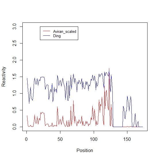
Reactivity profiles:

The figure generated shows that the two formulas yield different profiles.

Special cases that yield high correlation

In the absence of (-) channel noise (i.e., $Y_i=0$ for all $i$) and uniformity of coverage across the transcript (i.e., nucleotide-level coverage is equal for all nucleotides), we will see that both formulas would yield well-correlated profiles, if measuring correlation by Spearman rank correlation.

First, if we assume the absence of (-) channel noise and nucleotide-level coverage is equal for all nucleotides, both formula can be changed to the following format:

$\beta _k = max \Big( \frac{X_k}{c}, 0 \Big),\qquad$ (Aviran et al.)

$\beta_k = max \Big( \frac{ln(1+X_k)}{\frac{1}{n}\sum_{i=k}^{n+1} ln(1+X_i)}, 0 \Big),\qquad$ (Ding et al.)

where $c$ is a constant representing nucleotide-level coverage, $c=\sum_{i=k}^{n+1} X_i$.

Then we have the profiles changed as shown on the Figure1 (Note that red line is scaled by 30 fold for visualization convenience). The Spearman rank correlation calculated in R is 1, suggesting that in this case two profiles are highly correlated.

Differences between Spearman and Pearson Correlation

However, Pearson correlation is only 0.598, not as high as spearman. This is caused by the fact that Spearman correlation coefficient is based on the ranked values for each variable rather than the raw data. In general, Pearson measures linear relationships, and Spearman measures monotonic relationships. Two variables get high Pearson correlation coefficient when one variable is associated with a proportional change in the other variable. In contrast, two variables get high Spearman rank correlation coefficient when the variables tend to change together, but not necessarily at a constant rate.

Advantages of using Spearman: It can find the similarity in both methods, although it is not intuitive to judge from the profile figure. And easy to validate that Aviran’s methods can generate high reactivity estimate on the nucleotides where Ding’s method gave a high reactivity estimate.

Disadvantages of using Spearman: It neglect the fact that two methods generate very different scores in some positions, and the relationship is not proportional. Aviran’s method tend to have more peaks that exhibit much higher value than the surroundings, and tend to have a decay trend from right to left on the graph. This part of information is missed.

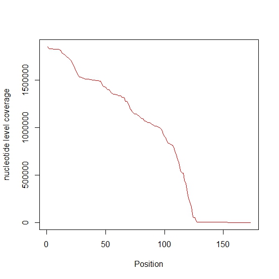
Nucleotide-level coverage

Nucleotide-level coverage profile for (+) channel of provided dataset is plotted below which shows that nucleotide-level coverage is not uniform in this dataset.

Log transformation

One thing we noticed is that, Ding’s method applies log transformation on the data. One justification for log transformation in the formula is that, the large value variation can be minimized to a smaller range.

Differences in paired-end and single-end sequencing approaches

We noticed that these two articles uses single-end sequencing and paired-end sequencing respectively. While paired-end sequencing captures accurate information, single-end sequencing is cheaper. In considering the requirements for accurate single-end sequencing, size selection is essential. Length selection, which can be performed by gel electrophoresis or magnetic beads, will help reduce the noise level in the experiment. We can also improve the accuracy of single-end sequencing by increasing the number of biological replicates in the experiment–more biological replicates improves the measure of variation in the experiment, leading to more accurate results. Somewhat similarly, we can consider increasing the number of technical replicates. Here, it is key to use the same platform for all measurements, in order to minimize any biases or other effects that could arise upon alteration of the experimental setup. Finally, we can ensure the best accuracy for single-end sequencing by increasing the read depth in our experiment. Gathering more reads provides better coverage of the sample and will help minimize error in sequencing.

Differences in single primer and random primers

In the SHAPE-Seq experiment that was modeled by Aviran et al., a single primer targeted at the 3’ end is used. One of the reasons for monotonic decrease in nucleotide-level coverage towards the 5’ end in pT181 dataset (which has been obtained in a SHAPE-Seq experiment) is that there was only one priming site. Reverse transcriptions are less likely to reach sites farther away from priming site, thus causing non-uniformity in coverage. To tackle this issue, Ding et al. used a random priming approach. This approach utilizes a pool of hexamers of all possible sequence combinations for priming. These 6 nt long primers could bind and initiate transcription at any site along the transcript, thus making nucleotide-level coverage more uniform. The random priming approach is accompanied by several challenges, since sites vary in their affinity for priming. First, consider the thermodynamic variation among sites: different sites have different values for the Gibbs free energy, and those with reduced free energy will be more likely to result in successful priming. As such, certain areas of the sample will be initiating priming more than others, leading to some variation in coverage. Additionally, there are structural considerations-primers are less likely to bind in loop regions, reducing the coverage within and slightly after these locations. Finally, the GC content within the sample will have an interesting effect on the random priming approach. Priming will be highly likely in regions that possess a high GC content, due to the strength of GC bonds.

Take-home messages

If uniformity of nucleotide-level coverage cannot be ensured, Aviran’s method is more accurate, as it considers nucleotide-level coverage in the summation. As such, the change of nucleotide-level coverage will be reflected in Aviran’s method, but not in Ding’s formulation. If low (-) channel noise cannot be ensured, Ding’s method will generate more reasonable values. Ding’s method utilizes a logarithm-based approach, which will mitigate any extreme noise values. Aviran’s approach, on the other hand, is derived based on low-noise assumption; as a result, it may overestimate the reactivity at high noise levels.

References:

1. Nature 505, 696-700 (30 January 2014) doi:10.1038/nature12756
2. PNAS July 5, 2011 vol. 108 no. 27 11069-11074