People have been utilize deep learning widely in health, wearable electronics, household appliance, cars, social networks and industry, but in the field of genomics, the magic has just emerged, despite the massive big data generated in this field.

In this blog, I will review a recent paper on Nature Biotechnology 2015$^1$, named Predicting the Sequence Specificities of DNA- and RNA-binding Proteins by Deep Learning published. I am personally interested in this article, because of two reasons. First, I recently worked with synthetic biologists to optimize the quantity of transcription factors, which belongs to DNA-binding proteins, and it helps me develop better understanding by studying the most advanced research about it. Second, I am curious about how to apply deep learning in DNA/RNA sequences in general, the advantages and obstacles.

Why deep learning?

As a matter of fact, researchers has been exploring different methods for predicting sequence specificities of DNA/RNA binding proteins, such as MatrixREDUCE, MEMERIS, Covariance models, and RNAcontext, etc. Then what we can gain from this deep learning method? I summarize the following reasons:

• It outperforms all the aforementioned methods with both in vivo and in vitro datasets in predicting DNA- and RNA- binding protein specificities.
• Ease of training across different measurement platforms, such as Protein-DNA Binding Microarray (PBM), Chromatin Immunoprecipitation (ChIP) Assays, and HT-SELEX.
• Parameter tuning is automatic, more generic and less labor intensive for new datasets.

How is Sequence Specificities Measured?

Before taking a look into the model, one need to get a basic idea about how those input datasets are generated. $^{9-13}$

PBM utilizes microarray chips where an array of capture DNA strands is bound, typically labelled by probe molecules. ChIP methods works by forming and isolating immuno-complex at the binding sites, which works well in vivo. SELEX (systematic evolution of ligands by exponential enrichment) is a method to enrich small populations of bound DNAs from a random sequence pool by PCR amplification.

Workflow

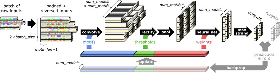
The overall workflow includes feed-forward stages and back-propagation stages. Feed-forward stages contains sequence conversion, convolution, rectification, pooling, and neural networks. We will talk about each in detail below.

Sequence Conversion

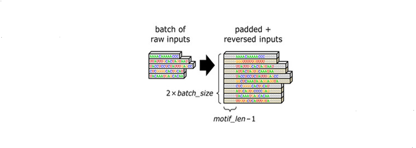
The first step is to convert the sequences in the datasets into proper mathematical representations. Let’s say we have n sequences as inputs. In this step, extra padding of length $m - 1$ is inserted at the head and tail of each sequence, permitting detection at extreme ends. $m$ is the length of motifs. Meanwhile, the number of input sequences doubles. Because typically when one sequence is measured with high DNA- or RNA-binding affinity, we are not sure whether it is the given strand or its reverse strand that is dominating. Thus both given sequences and their reverse strands are used as inputs for the following steps. Mathematically, the conversion formula is:

A sequence of ATGG can be represented as a matrix $S$:

Convolution

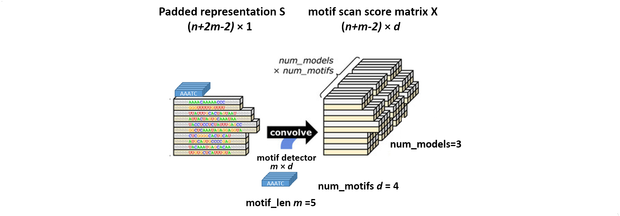
The padded representation matrix $S$ is then convolved with a motif detector array of $m \times d$. $d$ is the total number of motifs, while $m$ is the length of motifs. The motif detector array is randomly generated by a uniform sampler at the beginning of training. The convolution is done by sequentially aligning the motif detector array with each individual position on the sequence representation, followed by multiplication and summing. As a result, we get a high-dimensional motif scan score matrix $X \big( 2n \times \big( n + m - 2 \big) \times d \big) $. And mathematically 4 matrix representing A, T, C, and G are generated. More often than not, multiple models are trained in parallel (3 models in this figure).

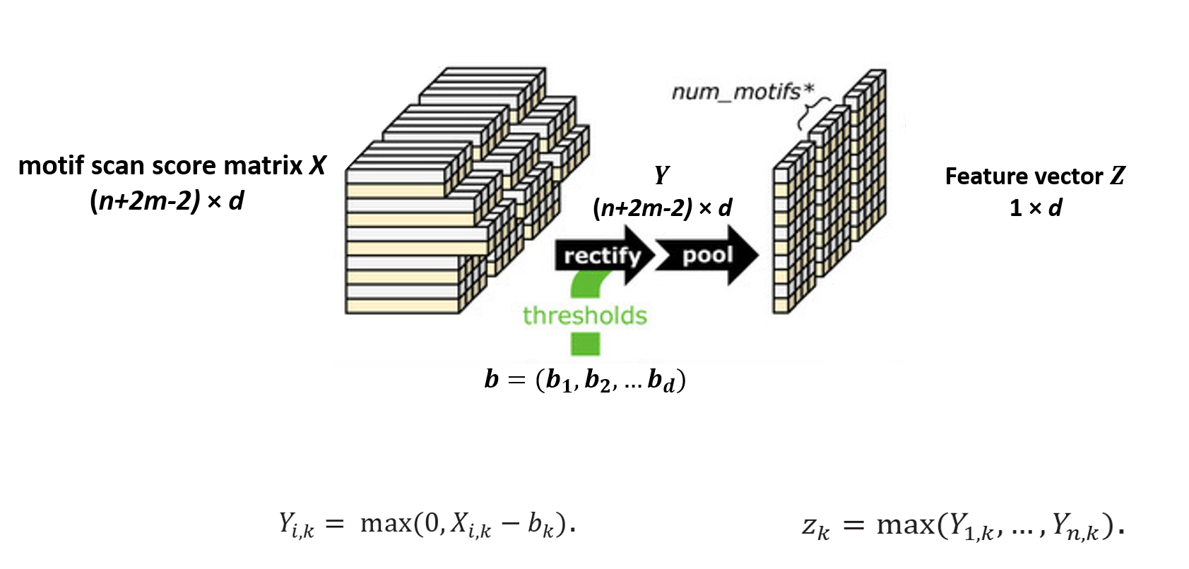
Rectification and Pooling

The rectification and pooling steps are quite straightforward. A vector of threshold values is given, corresponding to each motif. The convolution outcomes are compared with these thresholds, and negative ones are filtered out. The rectified matrix is represented by $Y$. However, there are still too many features in the matrix. To reduce complexity, we use a pooling step to extract features. The pooling step is done by taking the maximal value or average value of each vector in the convolution matrix, as a representation of the matching score of a motif to a sequence. Maximal values are used for DNA data, while both maximal and averaging values are used for RNA data, depending on which one has better performance. As a result, we get a feature vector $Z \big( 1 \times d \big) $ for each training model, to be used as an input of neural networks. For simplicity, we only use the pooling steps using maximal values to explain the following steps.

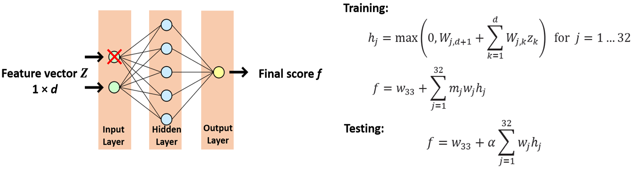
Neural Network with Dropout

A recent enhancement of neural networks known as dropout is illustrated here. The idea behind dropout is to occasionally “drop out” intermediate values (e.g. the $Z_k$ values) by randomly setting them to zero during training. Injecting this particular type of noise at training time cam prevent the neural network from over-fitting. The neural network used here is with one hidden layer that consist of 32 rectified units. During training, a binary mask variable $m \big( \sim Bernoulli \big( \alpha \big) \big) $ is assigned on each intermediate values. When $m$ is sampled as 0, this value is dropped out. However, in the testing step, we want to make the prediction consistent. Instead, the expected value $\alpha$ is used as a mask on the intermediate values. Our neural network has weight parameters represented by $w_k$.

Training Objectives

Our training objective is to minimize the following function $J$. This training objective is a combination of loss function and $L1$ normalization of weight decays. It has a trend to minimize the weights in neural networks $\big( W, w \big)$ and motif arrays ($M$), by giving a penalty parameter $\beta$, unless the loss function is good enough to pay for the penalties.

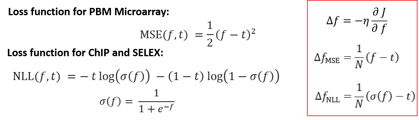
Loss function is generated by comparing the scores with experimental measures. Here because scores from ChIP and SELEX are either 0 or 1, while scores from PBM are not binary, we use different loss functions. As a result, when we do gradient descent, we have two forms of $\Delta f$.

Back-propagation Stages

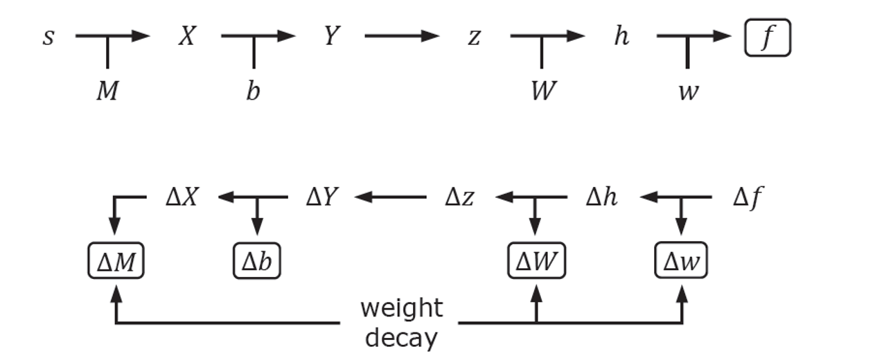
For detailed guidance on selection of loss functions and stochastic gradient descent, one can refer to Chapter 6 in Reference 2. We use gradient descent to optimize our parameters. As shown in this figure, the $\Delta$ values of each parameter can be calculated backwards from $\Delta f$ by the chain rule. For example, we can calculate $\Delta w$ from $\Delta f$ and $\frac{\partial f}{\partial w}$.

And all the rest $\Delta$ values can be calculated in a similar way. Eventually, all parameters are updated by their $\Delta$ values, and the training proceed iteration by iteration until the objective function converges to a certain threshold.

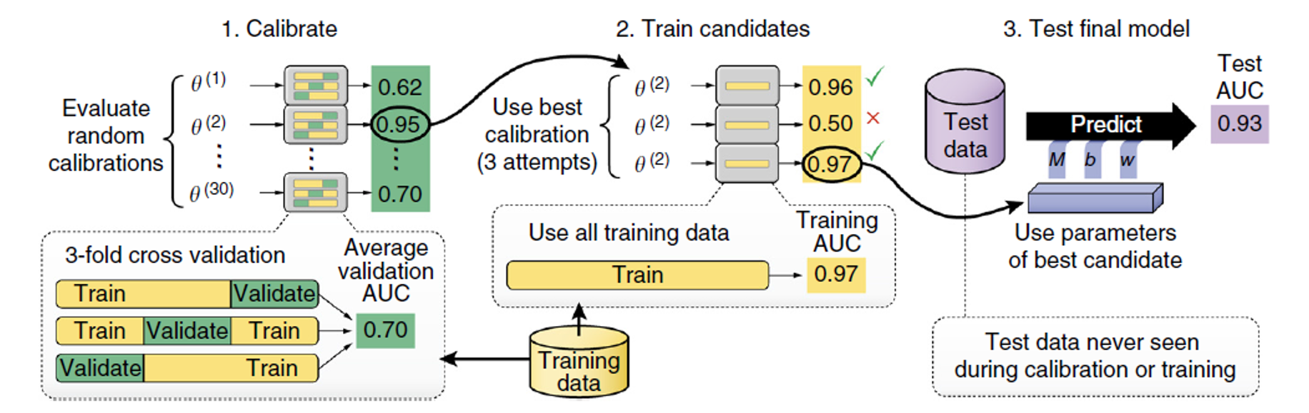
Automatic Parameter Calibration

One important work before start training any new datasets, is to calibrate the parameters. In this article, the calibration step is fully automatic, and it turns out to work well with random initialization. Our parameters include motif length $m$, motif numbers $d$, learning rate $\eta$, Learning momentum, batch size, weight decay $\beta$, dropout expectation $\alpha$, etc. First of all, 30 sets of parameters are randomly sampled, and trained in parallel with a 3-fold cross validation. The set of parameters with best performance is selected to train the entire training set on several parallel models. Multiple models training in parallel can help avoid random initialization effect and stochasticity of gradient descent. Eventually, the model with best performance is used in predicting new sequences.

Dataset Sizes and Shortcomings

In this article, separate models for over 2603 different protein binding data sets have been trained, the vast majority of which are large-scale ($\geq$ 10,000 sequences). Each data set requires its own calibration phase involving 30 trials, so tens of thousands of models are trained in total. To train these models in reasonable time, a specialized GPU-accelerated implementation of DeepBind has been built. However, it poses a unique challenge because the DeepBind models are much smaller (16 motif detectors, 32 hidden units) than comparable models used in computer vision. Modern GPUs are single instruction multiple data (SIMD) architectures, and their speed only comes by massive data parallelism, not by faster calculations. A straightforward GPU implementation of neural networks will only bring speedups for very large models, but DeepBind models are not individually large. The speed of a GPU comes from all these units executing in parallel, but it can only do so if each job sent to the GPU has enough work to keep the majority of these computational units busy. To leverage the power of GPUs in small-model scenarios, DeepBind training on the GPU is accelerated by training several independent models at the same time on the same GPU.

Conclusion

This article has done a great job balancing the number of models, complexity of models and parallel computing. It is very helpful to learn the ways they pre-process sequence data, extract features, and calibrate the parameters. Later this model has been used in identifying diseases-related variants in the sequences of DNA- and RNA- binding proteins, setting a great example for applying deep learning models in biomedical research.

---

References

1. Alipanahi, B., Delong, A., Weirauch, M. T., & Frey B. J., Nature Biotechnology 33, 831-838 (2015) doi:10.1038/nbt.3300
2. Duda, R. O., Hart, P. E. & Stork, D. G. Pattern Classification (2nd Edition, 2000).
3. Brivanlou AH, Darnell JE (Feb 2002). “Signal transduction and the control of gene expression”. Science. 295 (5556): 813-8.
4. https://www.biostars.org/p/53590/
5. RNA-Binding Proteins Impacting on Internal Initiation of Translation, Encarnacion Martinez-Salas, Gloria Lozano, Javier Fernandez-Chamorro, Rosario Francisco-Velilla, Alfonso Galan and Rosa Diaz, Int. J. Mol. Sci. 2013, 14(11), 21705-21726, doi:10.3390/ijms141121705
6. Direct measurement of DNA affinity landscapes on a high-throughput sequencing instrument Razvan Nutiu, Robin C Friedman, Shujun Luo, Irina Khrebtukova, David Silva, Robin Li, Lu Zhang, Gary P Schroth & Christopher B Burg, Nature Biotechnology, 29, 659-664 (2011), doi:10.1038/nbt.1882
7. Stormo, G. DNA binding sites: representation and discovery. Bioinformatics 16, 16-23 (2000).
8. Rohs, R. et al. Origins of specificity in protein-DNA recognition. Annu. Rev. Biochem. 79, 233-269 (2010).
9. Kazan, H., Ray, D., Chan, E.T., Hughes, T.R. & Morris, Q. RNAcontext: a new method for learning the sequence and structure binding preferences of RNA-binding proteins. PLoS Comput. Biol. 6, e1000832 (2010).
10. Nutiu, R. et al. Direct measurement of DNA affinity landscapes on a high-throughput sequencing instrument. Nat. Biotechnol. 29, 659-664 (2011).
11. Mukherjee, S. et al. Rapid analysis of the DNA-binding specificities of transcription factors with DNA microarrays. Nat. Genet. 36, 1331-1339 (2004).
12. Jolma, A. et al. Multiplexed massively parallel SELEX for characterization of human transcription factor binding specificities. Genome Res. 20, 861-873 (2010).
13. http://www.creative-biogene.com/Services/Aptamers/Technology-Platforms.html