
Differential Gene Expression Analysis of Adrenal and Brain Tissues
Differential Gene Expression, also known as DEG (Differentially expressed genes), is becoming a hot topic in fundenmental science research now, with the advancement of Next Generation Sequencing and single-cell isolation technology. In this blog, I will talk about the following topics:
- What is DEG and why it is so popular
- What is the differences between Cuffdiff, EdgeR, and DESeq2
- How to preprocess your data from the Sequencer
- How to get DEG analysis results usign R packages
- Visualization of DEG
Background
The original question is, if the genome is the same in all somatic cells within an organism (with the exception of the above-mentioned lymphocytes), how do the cells become different from one another? How come that your red bllod cells produce hemoglobin, while your cardiomyocytes controls your heart beating? The answer is differential gene expression.
Although every cell contains the same complete genome DNA, only a small percentage of the DNA is selectively expressed in each cell, therefore a specific portion of the RNA is synthesized in that cell type. For instance, if your body is a comparable to a country, then each cell is an individual person in this community. Before differential gene expression is studied, we only have the base knowledge of the country as a whole. The ultimate goal of differential gene expression is to obtain the portfolio the race, occupation, and personality of each individual.
Being able to recognize differential gene expression, is a key to understanding the specific roles that a cell is playing, or cell mutation. Thus it is becoming crucial for understanding the initial development of diseases, such as cancers and diabetes, growth of organs in childhood, as well as monitoring the influence of environment change. The expression level of each RNA unit is measured by the number of sequenced fragments that map to the transcript, which is expected to correlate directly with its abundance level.
Datasets
Here we analysis the differentially expressed genes in brain cells and adrenal cells. The datasets are paired-end 50bp FASTQ Sanger reads from adrenal and brain tissues (500Kb region of chromosome 19, chr19:3000000:3500000). These pair-ended sequencing data contains 4 Sanger reads file in total in FASTQ format, one forward reads and one reverse reads for each tissue. Each reads file contains around 50,000 short reads. You can download the datasets here: https://usegalaxy.org/u/jeremy/p/galaxy-rna-seq-analysis-exercise. But it is recommended to pre-process and map them to human genome on GALAXY first, since the raw data is a mess.
Algorithms and tools
In this blog, I will walk you through several algorithms that serve to answer the question that why cell from different tissues act differently, more specifically, which genes are expressed in one tissue but not in the other tissue.
GALAXY is a free public server for DEG analysis, which I have introduced in a previous blog. Here in this blog I will mainly introduce edgeR and DESeq2.
R packages for edgeR can be found here. http://www.bioconductor.org/packages/release/bioc/html/edgeR.html
R packages for DESeq2 can be found here. http://bioconductor.org/packages/release/bioc/html/DESeq2.html
Preprocessing
A Python framework, named HTSeq, can be used to process and analyze alignment results from high-throughput sequencing (HTS) assays, which can be downloaded here. https://pypi.python.org/pypi/HTSeq
After mapping with TopHat on Galaxy, we can directly download the .bam files from TopHat, as we talked about in previous blog. Then use the following command to pre-process .bam files into count matrix. A Linux or Mac system is required in this step. Windows package haven’t been made yet.
htseq-count -f bam Galaxy18_accepted_hits.bam chr19_gene_annotation.gtf>18_raw_count.txt
htseq-count -f bam Galaxy23_accepted_hits.bam chr19_gene_annotation.gtf>23_raw_count.txt
EdgeR DEG analysis
Data was normalized based across samples. Below is the R code used for EdgeR. There is no replication, setting dispersion to NA. Poisson model was used here for dispersion estimates.
library("systemPipeR")
library("edgeR")
raw.data <- read.table("Adrenal_Brain.txt", header= FALSE ) # change to TRUE
head(raw.data)
counts <- raw.data[, -1]
 #print(counts)
 rownames(counts) <- raw.data[ , 1 ]
 colnames(counts) <- c("Adrenal", "Brain")
head( counts )
#setup the object
cds <- DGEList( counts , group = colnames(counts) )
names( cds )
head(cds$counts)
#check normalization factors
cds$samples
#change normalization factors
cds <- calcNormFactors( cds )
cds$samples
cds$samples$lib.size<- cds$samples$lib.size* cds$samples$norm.factors
cds$samples
names( cds )
de.poi <- exactTest( cds , dispersion = 1e-06 , pair = c("Adrenal", "Brain") )

options( digits = 3 )
topTags( de.poi , n = 100 , sort.by = "logFC" )

#Write the DEG matrix into a file
write.table(res_top, file = "EdgeROutput_top100.txt",
append = FALSE, sep = "\t")
Top 100 DEG generated can be found here.
DESeq2 DEG analysis
First we need to setup a colData file for design formula in DeSeq2 analysis as follows:
| — | Parts |
|---|---|
| Adrenal | Adrenal |
| Brain | Brain |
Then we can import count data and colData as below, setup the object and do the analysis.
library("DESeq2")

countData <- read.table("Adrenal_Brain.txt", header= TRUE)   #import count matrix data generated by HTSeq
countData
#import the colData for design and DeSeq2
#https://bioconductor.org/packages/release/bioc/manuals/DESeq2/man/DESeq2.pdf

colData <- read.table("colData.txt", header= TRUE)
head(colData)

# Setup the DeSeq DataSet object
dds <- DESeqDataSetFromMatrix( countData = sampleTable, colData=colData, design=~Parts)
dds$Parts <- factor(dds$Parts, levels=c("Adrenal","Brain"))
#Build the Deseq object
dds <- DESeq(dds)
dds

res <- results(dds)
res

#Sort the results by log fold change
res_ordered <- res[order(-abs(res$log2FoldChange)),]
res_ordered

#Select the top 100
res_top <-res_ordered[1:100,]
res_top

#Filter rows where the one log fold change is NA
res_top <- res_top[!is.na(res_top$log2FoldChange),]
nrow(res_top)

#Write the DEG matrix into a file
write.table(res_top, file = "DeSeq2Output_ordered_top54.txt",
append = FALSE, sep = "\t")
My DESeq2 results of top 100 DEG can be found here.
Visualization by Venn Diagram
library(limma)
library(VennDiagram)
c1.data <- read.table("Top100DEGCuffDiff3.txt", header= TRUE, sep="\t" )
head(c1.data)
Cufdiff <- c1.data[,3]#["gene"]
Cufdiff
Cufdiff[order((Cufdiff))]

c2.data <- read.table("EdgeRTop100DEG.txt", header= TRUE, sep="\t" )
head(c2.data)
EdgeR<- c2.data[,1]

c3.data <- read.table("DeSeq2Output_ordered_top100.txt", header= TRUE, sep="\t" )
head(c3.data)
DeSeq2 <- c3.data[,1]

x1<-list()
x1$A <- as.character(Cufdiff)
x1$B <- as.character(EdgeR)
x1$C <- as.character(DeSeq2)

d12<-intersect(x1$A, x1$B)
d23<-intersect(x1$B, x1$C)
d13<-intersect(x1$A, x1$C)
d123<-intersect(d12,d23)

draw.triple.venn(100,100,100,length(d12),length(d23),length(d13),length(d123),category=c("Cuffdiff", "EdgeR", "DeSeq2"),euler.d=FALSE, scaled=FALSE)
Venn Diagram:
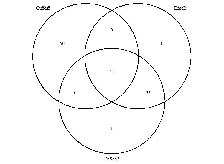
We can clearly tell from the Venn Diagram that EdgeR and DeSeq2 have high similarity in DEG analysis results. Only 1 gene out of 100 is different from these two sets, which is APOC4-APOC and APOC4-APOC2. However, Only 44% of Cuffdiff results overlap with either EdgeR or DeSeq2.
Insights for future DEG analysis
The reason is that Cuffdiff serves for different purposes comparing with the other two. Cuffdiff tries to identify the abundance of different transcripts across samples, assuming the experimental conditions are similar. However, EdgeR and DeSeq2 are tries to answer if the difference in total expression (total count of a gene including all its isoforms) you see between samples is solely due to experimental conditions or due to biological variance. Thus EdgeR and DeSeq2 are better at comparing multiple biological replicates. Also, the way to estimate dispersion parameters are different between Cuffdiff and EdgeR. Given more replicates, we can expect more similarity.
Thus Cuffdiff can be used for DEG analysis in samples with fewer replicates, and in cases where experimental conditions are the same. EdgeR and DeSeq2 can be used to deal with DEG analysis multiple experimental conditions controls.